Summation of Polynomials

Problem Name: Summation of Polynomials
UVa ID: 10302
Keywords: finite calculus, math

I have a real treat for you today. I am thrilled to have the opportunity to write about a fascinating topic I just learned about very recently. This post is supposed to be about problem 10302 from UVa’s archives, but it’s not simply about the specific solution to the problem, which is rather mundane, but about the theory behind it, which is introduced in the problem description.

It all started when I read this problem for the first time. If you haven’t done so yet, I suggest you go ahead and read it now. Read it a few times if necessary…

Ready? Okay, did you find anything particularly interesting there? If you managed to perfectly understand all that is being said there, I salute you, you are a true gentleman and a scholar. Personally, I found the problem description quite confusing, and the subtle errors (did you notice something funny in the definition of a factorial polynomial?) didn’t help. However, the concepts being described there had some strange appeal to me, so it motivated me to do some research on my own. I’m so glad I did! It allowed me to learn about this beautiful area of mathematics that you could call finite calculus (or discrete calculus).

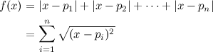
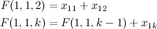
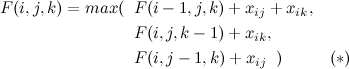
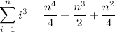
Before going any further, let’s quickly mention that the solution to this problem involves simply calculating the expression:

A simple search for “sum of consecutive powers” brings up countless documents that present the closed form expression to evaluate this sum:

We’ll come back to this later; for now, let’s go on with the topic at hand.

Finite Calculus - Calculus for computer scientists

Of course, people could disagree with this, but it seems to me that if you have any interest at all in computer science, there’s a good chance that you’ll find finite calculus deeply fascinating. For me, this was another instance of something that made me think “why didn’t they teach me this in school?!”. Maybe finite calculus is nothing new to you, and if that is the case, this post will be kind of boring, but if your academic education was somewhat similar to mine, you learned about the “traditional” branches of calculus: differential and integral calculus —which we’ll simply refer to as “infinite calculus” from here on— but you never heard about finite calculus.

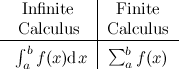
Well, I’m not claiming that this article will teach you everything there is to know about it, but it may be a good starting point. Let’s start with the basics; as their names suggest, infinite calculus and finite calculus are sub-fields of Calculus, but they differ in a very fundamental way. Infinite calculus concerns itself with curves, sums of infinite terms and functions that exist in the realm of the real numbers, while finite calculus is more interested in sequences, sums of a finite number of terms and functions that live in the space of integers. The following figure oversimplifies things, but illustrates the kind of things that each type of calculus focus on:

One of the most emblematic examples of a function relevant to our discussion that shows up frequently in computer science and discrete mathematics in general is the sum of the first \(n\) positive integers:

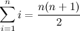
In fact, I’d say that if you’re reading these lines, it’s very likely that you already know the equation above by heart (and, maybe just as likely, you have heard the charming story about young Gauss and how he amazed his teacher by using a brilliant reasoning related to that formula). However, can you say that you are equally capable of formulating closed form expressions for the following sums, without any help from books or other sources?

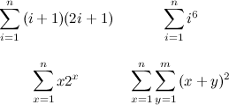
Well, if you are currently unable to answer affirmatively, rejoice, because you’re about to learn a nice approach to tackle these problems. I want to emphasize that this article is meant to be a simple introduction to finite calculus, but you can find a more complete document in the tutorial referenced at the end. I strongly recommend that you read it in its entirety for a more detailed explanation on many of the things mentioned here.

Definitions

Let’s get started (about time!). What we’ll see here is how, even though the basic definitions in finite calculus are necessarily different than the things you already know from infinite calculus, they closely relate to their infinite counterparts. Because of this, if you already know the basics of infinite calculus, learning finite calculus will be a breeze.

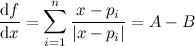
We’ll begin with the discrete derivative:

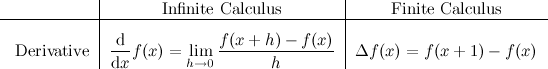
In discrete mathematics, the closest we can get to 0 (from the right) without touching it is 1, which gives us the simple expression above. \(\Delta\) is the finite difference operator, which in this case simply represents the difference between the value of a function evaluated at some point \(x\), and its value when evaluated one step above \(x\). This should give you an idea as to why the problem description talks about “anti-differences”, and why its definition looks the way it does.

Next, let’s see one of the most basic operations which we’ll use repeatedly from now on, the exponentiation or “power” function:

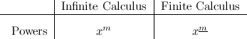
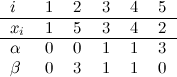
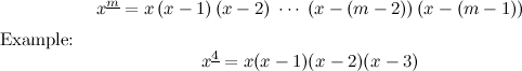
What is \(x^\underline{m}\)? It’s a “falling power” (the problem description calls it a factorial polynomial):

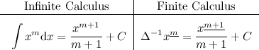
Why use such a strange type of “power”? Well, it will become clear when you see how the “derivatives” of polynomials work in finite calculus:

Isn’t that neat? Now that we have covered the basic of “finite differential calculus”, let’s see a little bit of “finite integral calculus”, which is what we’ll ultimately apply to solve the summations formulated above.

A function \(g(x)\) is called the discrete anti-derivative, or anti-difference of \(f(x)\) if \(\Delta g(x) = f(x)\):

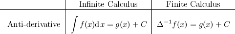
Here I have chosen \(\Delta^{-1}\) to denote the discrete anti–derivative. A different notation is used in the tutorial referenced at the end, but the meaning is the same. Notice that the similarities with infinite calculus still hold:

The last crucial element is to formulate something similar to the fundamental theorem of calculus, but for the discrete world:

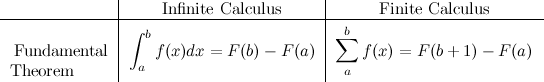
Where \(F(x)\) represents the anti–derivative of \(f(x)\). All of these elements give use enough tools to tackle our original problem, but before moving on to the examples, I want to mention a few more properties and relations that have elegant discrete counterparts (click on the image).

I find particularly interesting that the discrete counterpart of \(e\) is 2. If you are into computer science, I don’t need to explain how perfect that is.

Worked Example #1

Okay, let’s try applying all of this theory in a real problem. Let’s get back to our original summation:

How to solve this? Well, the fundamental theorem tells us that if we knew the anti–difference of \(x^3\) (let’s call it \(g(x)\)), then calculating the sum would be a matter of evaluating \(g(n+1) - g(1)\).

But to find \(g(x)\), first it would be convenient if we could express \(x^3\) as a sum of falling powers (a factorial polynomial):

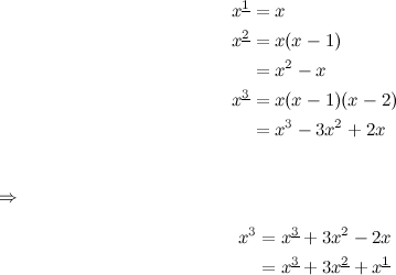
With this, finding the anti–difference is very easy:

Verifying that \(g(n+1)-g(1)\) is equal to the closed form formula presented at the beginning of this article is left as an exercise to the reader.

Worked Example #2

We’ll consider now the following summation (taken from the tutorial referenced below), which illustrates the use of “integration by parts” in finite calculus:

The key observation here is that, thanks to the multiplication of derivatives property, we can formulate the following relation —again, notice the striking similarity with infinite calculus:

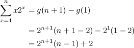
We’ll choose \(u(x)=x\) and \(\Delta v(x)=2^x\), which helps us find the anti–difference we want:

Finding the closed form expression for the sum is now trivial:

Really nice, isn’t it?

---

We have reached the end of this short introduction to the world of discrete calculus, and all that is left for me is to thank the problem setter for writing this problem specifically to introduce many of us to these fascinating mathematical ideas. See? This is one of the reasons why I love solving algorithm problems; every once in a while you come across a gem like this that helps you learn new and exciting stuff, and isn’t learning the point of all this? :)

References

• David Gleich. Finite Calculus: A Tutorial for Solving Nasty Sums. 2005. http://www.cs.purdue.edu/homes/dgleich/publications/finite-calculus.pdf

Bubbles and Buckets

Problem Name: Bubbles and Buckets
UVa ID: 11495
Keywords: sorting, inversion number

Since my previous post was about a problem that can be solved with a variation of a classic sorting algorithm, I thought it would be nice to do a follow–up with another problem that can also be solved by using a sorting algorithm as a basis.

In this problem it is said that two boys play a simple game: a random permutation of the first \(N\) positive integers is given, and then the two players take turns to make a move. A valid move consists of taking any pair of adjacent numbers that are in the wrong order (the first number is higher than the second), and swapping them. The player who can’t make a move (which means the list is completely sorted) loses. The question is, knowing the initial permutation, and the player who goes first, who wins?

Clearly, the core of this problem is finding the number of swaps between adjacent elements required to sort the list. If you don’t know how to find this value yet, take some time to look at the samples, and think about possible strategies to do it. You should be able to identify a few interesting invariants soon. For example: an indication of how far a number \(x_i\) is from its correct position is the amount of numbers larger than \(x_i\) that are located to its left, or the amount of numbers smaller than \(x_i\) that are located to its right. Let’s consider the first test case from the sample input:

In the table, \(\alpha\) represents the amount of numbers bigger than \(x_i\) that are left of the given number, and \(\beta\) is the amount of numbers smaller than \(x_i\) that are found to its right. As you can see, the sums from the \(\alpha\) and \(\beta\) rows are equal. That’s an invariant, and it’s related to the algorithm that we will ultimately use to calculate the answer.

Another way to look at it is this: \(\alpha\) and \(\beta\) are the amount of swaps that every number has to go through to sort the list. \(\alpha\) corresponds to swaps from right to left, and \(\beta\) to swaps from left to right. No matter the orientation of the swaps you choose, the total number of swaps will always be the same. In discrete mathematics, this is also known as the inversion number of a sequence.

Now, how to calculate this efficiently? Note that there can be up to \(10^5\) numbers in the list, so any kind of \(O(n^2)\) algorithm wouldn’t work. Well, we can just choose any of the \(O(n \log{n})\) sorting algorithms and adapt it to keep track of the number of times a swap in one particular direction has to be performed. One particularly good alternative is merge sort because of its simplicity, in contrast to something like quick sort, where —depending on your implementation and the way you handle the pivot— figuring out the number of swaps required when a number has to change its place can be significantly harder.

Having settled on the algorithm to use, let’s see an example of the implementation of merge sort for this problem:

typedef long long    i64;
typedef vector<int>  IV;
typedef IV::iterator IVi;

i64 n_swaps;  // the number of swaps can be very large

// auxiliary function used by merge_sort
void merge(IVi lo, IVi hi, IVi mid)
{
    IV x;
    for (IVi a = lo, b = mid; a < mid || b < hi; ) {
        if (a >= mid) { x.push_back(*b++); continue; }
        if (b >= hi) { x.push_back(*a++); continue; }
        if (*a < *b) { x.push_back(*a++); continue; }

        x.push_back(*b++);

        // here is the problem-specific adjustment
        // what does (mid - a) correspond to?
        n_swaps += mid - a;
    }
    for (IVi a = lo, b = x.begin(); a < hi; ++a, ++b)
        *a = *b;
}

// merge sort algorithm, receives iterators to the first (inclusive)
// and last (exclusive) elements of the range to sort
void merge_sort(IVi lo, IVi hi)
{
    if (hi <= lo + 1) return;
    IVi mid = lo + ((hi - lo) / 2);
    merge_sort(lo, mid);
    merge_sort(mid, hi);
    merge(lo, hi, mid);
}

---

For a similar problem —the algorithm is exactly the same, the main difference is that you have to print the number of swaps— see the problem Ultra-QuickSort (UVa ID 10810). Another similar problem, but with lower constraints (enough to make a \(O(n^2)\) solution feasible) is Flip Sort (UVa ID 10327).

Aladdin and the Optimal Invitation

Problem Name: Aladdin and the Optimal Invitation
LightOJ ID: 1349
Keywords: math, median, sorting, recursion, quickselect

Sometimes you come across a problem that forces you to look into new, interesting algorithms, which is always an excellent opportunity to extend your bag of tricks as a programmer, and can give you a new level of understanding of classic algorithms you take for granted. This problem is a good example.

You are given a rectangular matrix of integers, representing a town, where the integer values of each cell represent the amount of people living on that cell. You are asked for a particular position inside the matrix, such that the total sum of Manhattan distances of all people relative to that position is minimised. One thing you can quickly notice is that in this 2D problem you can consider each axis independently and combine the horizontal and vertical cases for your final answer.

Now, let’s think abstractly about the problem in one dimension; that is, given a set of 1-dimensional coordinates, find an optimal coordinate such that the total sum of distances from each point of the set to that optimal position is minimal. If you have come across this type of problem before, you probably know already that the answer is the median of the set of points. In case it’s not clear why, let’s stop for a moment and try to find a satisfying explanation:

~~~ math intermission ~~~

Let’s express the total sum of distances of all the points in the set to an arbitrary position \(x\) as a function:

Where \(p_i\) is each point from the set, and \(n\) is the number of points. Now, doing some mathematical optimisation, we find the first derivative of \(f\):

Where \(A\) is the number of points above \(x\), and \(B\) is the number of points below \(x\). The function \(f\) is minimal when its first derivative equals zero, which happens when the amount of points above \(x\) is the same amount of points below \(x\), or, in other words, when \(x\) is the median of the set of points. Note that there could be more than one value of \(x\) that satisfies the relation, which is consistent with the fact that the median is ambiguous when the number of points is an even number.

~~~ end of intermission ~~~

Solving this type of problem for relatively small data samples is very straightforward, just store the points in a list, sort the list, and find the value in the middle. For an example of a programming problem that can be solved this way, see Vito’s Family (UVa ID 10041). However, the constraints in this problem make it impossible to solve it with that approach. There can be \(5 \times 10^4\) populated cells in the matrix, and a maximum of \(10^4\) people can live on each cell.

One way to solve this is using an algorithm known as “quick select”. A good explanation on this algorithm can be found here: Selection and order statistics. You don’t have to read the whole article, but at least make sure to glance over the “Quick select” and “Analysis of quickselect” sections.

You can think about it as a variation of the standard quick sort algorithm. In quick sort you receive a list of values, choose one of them as a pivot and then partition the list into three groups: the values to the “left” of the pivot, the values to the “right” of the pivot, and the pivot itself. If any of the left of right groups is not empty, you then call quick sort recursively on them. Quick select is very similar, but the difference is that its purpose is not sorting the list, but finding an arbitrary element in the list (let’s call it the \(k\)th position).

So the algorithm chooses a pivot (just like quicksort), partitions the list, but then it simply does the following checks:

• If the left group has at least \(k\) elements, then the \(k\)th element must be found there, so call quickselect recursively on that group.
• If the pivot is exactly the \(k\)th element, then the pivot has to be returned.
• Otherwise, the answer must be found on the right group, so make the recursive call on that.

In a way, this algorithm is simpler than quick sort because it doesn’t need to make recursive calls for the groups where it knows that the \(k\)th element is not going to be found. With all of this in mind, now let’s see a C++ implementation of quick select specifically tailored for this problem, heavily based on the pseudo-code for the “in-place” version of quick sort from Wikipedia.

struct Data {
    int v;  // value of data point (one-dimensional coordinate)
    int n;  // number of occurrences (people on that coordinate)
    int p;  // a sequential number, to break ties

    Data(int V, int N, int P) : v(V), n(N), p(P) {}

    bool operator<(const Data &x) const {
        if (v != x.v) return v < x.v;
        if (n != x.n) return n < x.n;
        return p < x.p;
    }
};

// we will use STL's vector
typedef vector<Data> DV;
typedef DV::iterator DVi;

/**
 * Selects an arbitrary position from a range of data, according
 * to its logical order. It modifies the vector in-place.
 *
 * @param lo The iterator to the first element in the range (inclusive)
 * @param hi The iterator to the last element (exclusive)
 * @param k  Index of the element to return (starting with 0)
 *
 * @return The kth element in order from the range of data
 */
int select_kth(DVi lo, DVi hi, int k)
{
    // if there is only one element left, it must be the answer
    if (hi == lo + 1) return lo->v;

    // choose a pivot at random
    int pivot_index = rand() % (hi - lo);

    // move the pivot to the last position
    swap(*(lo + pivot_index), *(hi - 1));

    // keep the pivot's value at hand
    Data piv = *(hi - 1);

    // iterator to keep track of the "left" group
    DVi x = lo;

    // number of people that has gone to the "left" group
    int lt = 0;

    // traverse the range of data
    for (DVi i = lo; i < hi - 1; ++i)
        if (*i < piv) {
            // if the current element belongs to the left group ..

            swap(*i, *x);  // move it to the tail pointed by x
            lt += x->n;    // increase the number of people
            ++x;           // move the x iterator
        }

    // move the pivot back to its rightful place
    swap(*x, *(hi - 1));

    // if k is found in the left group
    if (k < lt)
        return select_kth(lo, x, k);

    // if k is greater than the amount of people in the left group
    // and the pivot
    if (k >= lt + x->n)
        return select_kth(x + 1, hi, k - lt - x->n);

    // the only possibility now is that k is in the pivot
    return x->v;
}

As you can see, it follows the quick sort pattern very closely, but it doesn’t bother sorting the entire list, just locates the \(k\)th element.

A couple of details are worth noting: the use of an extra field (p) in the Data structure (line 4), and the selection of the pivot at random (line 35). Both are related to the same issue: performance. If you read the comments on the performance of this algorithm in the article cited above, you realise that it can have a \(O(n^2)\) complexity for a worst case, but it is asymptotically optimal if the pivots are chosen carefully.

I actually came across this issue while testing my solution. Consider a test case with \(q=50000\), where \(u\) and \(v\) are always the same, and \(w\) is always \(10000\). If we always choose the pivot to be, let’s say the first element of the range, then it’s clear that on each call of the select_kth function the “left” group will be empty, and it will keep calling itself after discarding only one element from the list (the pivot). Clearly in this case it will perform very badly.

However, by always choosing the pivot randomly, and by making sure that the Data points can always be sorted unambiguously, the “left” groups will be of an average size, and the total complexity gets reduced drastically.

---

I really liked how this problem shows that, even if you would very rarely need to write a quick sort function (using the implementation from your programming language is a much better idea), knowing its inner workings is very useful to implement variations like quick select, which has the potential to provide elegant solutions in problems related to selecting elements from large lists.

Treblecross

Problem Name: Treblecross
UVa ID: 10561
LightOJ ID: 1229
Keywords: game theory, impartial game, sprague-grundy numbers

Quoting from the problem description:

Treblecross is a two player game where the goal is to get three X in a row on a one-dimensional board.

This can be recognised as a finite impartial game (finite meaning that it is not possible to keep playing it forever). This means that it can be analysed using the Sprague–Grundy theorem. This is very much related to the game of nim and many other impartial games. For those who are not yet familiar with these topics I can highly recommend the following article that does an excellent job explaining the basics of it: Sprague–Grundy theory.

What makes this problem interesting is that it’s one of those cases where the method to apply the Grundy theory is not very apparent at first, because it doesn’t look very much like just another variant of the classic nim game. And yet, the theory tells us that is should be possible to transform this game’s rules into something that can be modelled as a combination of nim games. Let’s try to do that.

But before going into the main rules, let’s stop for a second to notice one important thing: the problem gives us an arbitrary configuration for a game (which could be after having played a few rounds), and we have to identify all position from which a win is possible, given that both players play optimally. This is significant for one reason, which is that, unlike a fresh new game, an arbitrary game configuration could have trivial win positions. By trivial win positions I’m referring to any positions where placing an X ends the game with a win for the first player in just one move. Those positions don’t really fit into the theory discussed further below, so we better handle those as special cases right away. For example, in the following test case:

Positions 4, 7 and 10 are trivial wins. With that out of the way, we can concentrate on a game without trivial wins, which makes it possible to apply the Grundy number theory.

Let’s consider the following example:

One notable observation is this: an ideal move would never be done on a position closer than 3 cells to any X already on the board. In the example above, placing an X into any position other than 6 will give the opponent a trivial win. So, we consider any position at a distance of 1 or 2 to the closest X as unplayable, and now we see that the first player has only one possible move which is the 6. In fact, that move guarantees a win, because no matter what the other player does next, it will give us a trivial win in the following turn.

This already gives us a major piece of the puzzle of how to transform any arbitrary treblecross game, into a nim game. Let’s describe a treblecross game as a sequence of integer numbers that represent the length of all “open intervals” in the board in order. For example, the previous example would be denoted \((2, 5, 2)\). The other major piece of the puzzle is this: an open interval of length \(L\) is equivalent to a single treblecross game with a clean board of size \(\text{max}(0, L - 2x)\) where \(x\) is the number of X’s that surround the open interval. For example, the open interval 1 to 2 has 1 surrounding X, while the interval 4 to 8 has 2.

So, the game \((2, 5, 2)\) is equivalent to the combination of three separate games \(\{ (0), (1), (0) \}\) and, as the game theory tells us, if we know the “nim number” or nimber of each separate game, then we can know the nimber of their combination by simply applying the XOR operation.

All that is left now is calculating the S.G. numbers (or nimbers, as we have called them) of all possible “clean board” games of treblecross. Here’s a table that includes the first few cases:

To come up with this table, you just have to notice that placing an X anywhere on a clean board splits the game into two. The second column of the table has the list of reachable configurations, which are the games that can result after a single move from the game in the first column. Note how the \((4)\) game is the first one to reach a configuration with a \((1)\), because of the \(\text{max}(0, L - 2x)\) rule. The way those reachable positions are combined and how the new nimber is selected by applying the S.G. theorem is left as an exercise to the reader.

To summarise, the solution to this problem involves calculating the S.G. numbers of treblecross games of all sizes up to 200. Then, for each test case, the open intervals have to be identified, and then for each position with a dot, you calculate what would be the resulting intervals if an X would be placed there, and that gives you a new nimber. If that nimber is 0, then that position has to be printed, because the game is winnable from there. Make sure, however, not to include positions that give trivial wins to the next player. For example, in the game \((2, 5, 2)\) discussed above, if you place an X on position 5, you would find that the resulting intervals are \((2, 1, 3, 2)\) which you might turn into the combination of games \(\{ (0), (0), (0), (0) \}\), which has the nimber 0. But that position is not a good move because it gives a trivial win to the opponent.

One last tip. To simplify the calculation of the intervals with the \(\text{max}(0, L - 2x)\) rule, you can imagine an extended board, with three additional positions at each end. And then place an X on the very first and last positions of that extended board. Then the conversion of all intervals into a single treblecross game would be simply \(\text{max}(0, L - 4)\).

Baker Vai

Problem Name: Baker Vai
LightOJ ID: 1071
Keywords: dynamic programming

One thing that I have heard and read numerous times about dynamic programming, and I completely agree with this, is that no matter how much experience you have solving problems using D.P., there’s always the chance that a new problem shows up that makes you stop and think hard about how to solve it. When that happens, it’s a beautiful thing, because you get the chance to expand the problem solving framework in your mind a little bit and get new inspirations on how to tackle problems in the future.

I liked this problem because it was one of those cases for me. The problem asks for the maximum sum possible when moving inside a matrix of integers of size \(m \times n\). You start on the top-left corner, and moving only down or right you have to reach the bottom-right corner, and then go back to where you started, moving only up or left. In addition, you can’t step on any cell more than once, except for the point where you started.

One thing that usually helps is trying to model the problem as something “simpler”, but equivalent (simpler is, of course, a matter of perception and it works differently for different people). Here’s how I thought about this; consider a matrix of size \(m \times n\):

The problem is equivalent to finding two disjoint paths \(P_L\) and \(P_R\) (representing a left path and a right path), such that \(P_L\) starts at position \((1,1)\) and ends at \((m,n-1)\), and \(P_R\) starts at \((1,2)\) and ends at \((m,n)\):

The paths have to be built with only two kinds of movement, right or down, and the sums of the cells they visit have to be maximum. Can you see how this is equivalent to our original problem?

There are a few interesting invariants that apply to this model, very similar to the ones that apply to the easier problem of solving this just for one path. For example, both \(P_L\) and \(P_R\) will have exactly \((m-1)\) down movements and \((n-2)\) right movements.

Let’s try to define our D.P. relation now:

\(F(i, j, k)\)

The maximum sum possible after reaching the \(i\)th row, where \(P_L\) is on column \(j\), and \(P_R\) is on column \(k\).

The base case is the first row:

Now, for the rest of the rows, we’ll consider three cases: both paths go down one step at the same time, or \(P_L\) moves to the right, or \(P_R\) moves to the right:

Note that the expression in the line marked with (*) has a special caveat: it can only be considered if \(x_{i j}\) is not part of \(P_R\). Otherwise, you may count some cells twice, and that would produce the wrong results.

For example, consider the following pseudo-code for the above relation:

dp[M][N][N] is the D.P. data structure

for each i from 2 to M:
    for each j from 1 to N-1:
        for each k from j+1 to N:

            // calculate the new DP value
            val := dp[i-1][j][k] + x[i][j] + x[i][k] ;

            val := max(val, dp[i][j][k-1] + x[i][k]) ;
            val := max(val, dp[i][j-1][k] + x[i][j]) ;

            dp[i][j][k] := val ;

        end for;
    end for ;
end for ;

This code has the bug of not taking into account the caveat mentioned above. The order in which the columns \(j\) and \(k\) are visited by the loops don’t guarantee that x[i][j] hasn’t been counted already for dp[i][j][k-1].

How to fix it? Well, you can think about it like this: imagine that you use a chessboard of size \(m \times n\), and place two pawns in positions \((1,1)\) and \((1,2)\), and with them you simulate the movements of \(P_L\) and \(P_R\). One way to guarantee a correct sequence of movements is this:

• Let’s say that the two pawns are on row \(i\), and columns \(j\) and \(k\). First, move only the left pawn (the one at column \(j\)) to the right a certain number of times (but its final column has to be less than \(k\)).
• Then move only the right pawn to the right, any number of times (without going out of the board).
• Finally, if \(i < m\), move the two pawns down and go back to the first step.

That’s it. The way to avoid the counting cells more than once problem is in the order of our calculations.

The following pseudo-code illustrates a correct way of calculating the D.P. values for the rows 2 to \(m\):

for each i from 2 to M:

    // First consider only the down movement
    for each j from 1 to N-1:
        for each k from j+1 to N:
            dp[i][j][k] := dp[i-1][j][k] + x[i][j] + x[i][k] ;
        end for;
    end for ;

    // Now, move the left path only
    for each j from 2 to N-1:
        for each k from j+1 to N:
            dp[i][j][k] := max(dp[i][j][k], dp[i][j-1][k] + x[i][j] ;
        end for;
    end for ;

    // Finally, move the right path only
    for each j from 1 to N-2:
        for each k from j+2 to N:
            dp[i][j][k] := max(dp[i][j][k], dp[i][j][k-1] + x[i][k] ;
        end for;
    end for ;

end for ;

Note how in this pseudo–code, the indices for the D.P. matrix go from 1 to M and 1 to N, and how the loops are slightly different according to the situation.

References

Friday 13 July 2012